ICT Development Index 2010
Data Tables, Statistical Modelling, Information Technology, Economics
Date posted: 23 March 2012
The International Telecommunication Union (ITU) is a United
Nations agency responsible for information and communication
technology (ICT). The
ITU have published several ICT related indices, including an ICT
Development
Index
(IDI) and an ICT Price Basket (IPB) for most countries.
The IDI is a composite of 11 indicators, and is used to
compare the overall level of ICT development between countries. The IDI has three
sub-indices based on ICT access, use and skills.
The IPB is a composite basket based on the
prices for fixed
telephone, mobile cell-phone, and fixed broadband internet services,
expressed
as a percentage of average income levels.
The indices
were first published by the ITU in 2009, using 2008
data. At the time
of writing, the most
recent versions were published in 2011, and based on 2010 data.
ICT Development Index
(IDI) by Country
| Country |
IDI
2010 Rank |
IDI 2010 |
IDI
2008 Rank |
IDI 2008 |
| Korea (Rep.) |
1 |
8.40 |
1 |
7.80 |
| Sweden |
2 |
8.23 |
2 |
7.53 |
| Iceland |
3 |
8.06 |
7 |
7.12 |
| Denmark |
4 |
7.97 |
3 |
7.46 |
| Finland |
5 |
7.87 |
12 |
6.92 |
| Hong Kong, China |
6 |
7.79 |
6 |
7.14 |
| Luxembourg |
7 |
7.78 |
4 |
7.34 |
| Switzerland |
8 |
7.67 |
9 |
7.06 |
| Netherlands |
9 |
7.61 |
5 |
7.30 |
| United Kingdom |
10 |
7.60 |
10 |
7.03 |
| Norway |
11 |
7.60 |
8 |
7.12 |
| New Zealand |
12 |
7.43 |
16 |
6.65 |
| Japan |
13 |
7.42 |
11 |
7.01 |
| Australia |
14 |
7.36 |
14 |
6.78 |
| Germany |
15 |
7.27 |
13 |
6.87 |
| Austria |
16 |
7.17 |
21 |
6.41 |
| United States |
17 |
7.09 |
17 |
6.55 |
| France |
18 |
7.09 |
18 |
6.48 |
| Singapore |
19 |
7.08 |
15 |
6.71 |
| Israel |
20 |
6.87 |
23 |
6.20 |
| Macao, China |
21 |
6.84 |
27 |
5.84 |
| Belgium |
22 |
6.83 |
22 |
6.31 |
| Ireland |
23 |
6.78 |
19 |
6.43 |
| Slovenia |
24 |
6.75 |
24 |
6.19 |
| Spain |
25 |
6.73 |
25 |
6.18 |
| Canada |
26 |
6.69 |
20 |
6.42 |
| Portugal |
27 |
6.64 |
29 |
5.70 |
| Italy |
28 |
6.57 |
26 |
6.10 |
| Malta |
29 |
6.43 |
31 |
5.68 |
| Greece |
30 |
6.28 |
30 |
5.70 |
| Croatia |
31 |
6.21 |
36 |
5.43 |
| United Arab
Emirates |
32 |
6.19 |
32 |
5.63 |
| Estonia |
33 |
6.16 |
28 |
5.81 |
| Hungary |
34 |
6.04 |
34 |
5.47 |
| Lithuania |
35 |
6.04 |
35 |
5.44 |
| Cyprus |
36 |
5.98 |
43 |
5.02 |
| Czech Republic |
37 |
5.97 |
37 |
5.42 |
| Poland |
38 |
5.95 |
41 |
5.29 |
| Slovak Republic |
39 |
5.94 |
40 |
5.30 |
| Latvia |
40 |
5.90 |
39 |
5.31 |
| Barbados |
41 |
5.83 |
33 |
5.47 |
| Antigua
& Barbuda |
42 |
5.63 |
38 |
5.32 |
| Brunei
Darussalam |
43 |
5.61 |
44 |
4.97 |
| Qatar |
44 |
5.60 |
48 |
4.50 |
| Bahrain |
45 |
5.57 |
42 |
5.16 |
| Saudi Arabia |
46 |
5.42 |
55 |
4.13 |
| Russia |
47 |
5.38 |
49 |
4.42 |
| Romania |
48 |
5.20 |
46 |
4.67 |
| Bulgaria |
49 |
5.19 |
45 |
4.75 |
| Serbia |
50 |
5.11 |
47 |
4.51 |
| Montenegro |
51 |
5.03 |
50 |
4.29 |
| Belarus |
52 |
5.01 |
58 |
3.93 |
| TFYR Macedonia |
53 |
4.98 |
52 |
4.20 |
| Uruguay |
54 |
4.93 |
51 |
4.21 |
| Chile |
55 |
4.65 |
54 |
4.14 |
| Argentina |
56 |
4.64 |
53 |
4.16 |
| Moldova |
57 |
4.47 |
64 |
3.57 |
| Malaysia |
58 |
4.45 |
57 |
3.96 |
| Turkey |
59 |
4.42 |
60 |
3.81 |
| Oman |
60 |
4.38 |
68 |
3.45 |
| Trinidad
& Tobago |
61 |
4.36 |
56 |
3.99 |
| Ukraine |
62 |
4.34 |
59 |
3.83 |
| Bosnia
and Herzegovina |
63 |
4.31 |
63 |
3.58 |
| Brazil |
64 |
4.22 |
62 |
3.72 |
| Venezuela |
65 |
4.11 |
61 |
3.73 |
| Panama |
66 |
4.09 |
67 |
3.52 |
| Maldives |
67 |
4.05 |
66 |
3.54 |
| Kazakhstan |
68 |
4.02 |
72 |
3.39 |
| Mauritius |
69 |
4.00 |
70 |
3.43 |
| Costa Rica |
70 |
3.99 |
69 |
3.45 |
| Seychelles |
71 |
3.94 |
65 |
3.56 |
| Armenia |
72 |
3.87 |
86 |
2.94 |
| Jordan |
73 |
3.83 |
73 |
3.29 |
| Azerbaijan |
74 |
3.78 |
83 |
2.97 |
| Mexico |
75 |
3.75 |
74 |
3.26 |
| Colombia |
76 |
3.75 |
71 |
3.39 |
| Georgia |
77 |
3.65 |
85 |
2.96 |
| Albania |
78 |
3.61 |
81 |
2.99 |
| Lebanon |
79 |
3.57 |
77 |
3.12 |
| China |
80 |
3.55 |
75 |
3.17 |
| Viet Nam |
81 |
3.53 |
91 |
2.76 |
| Suriname |
82 |
3.52 |
78 |
3.09 |
| Peru |
83 |
3.52 |
76 |
3.12 |
| Tunisia |
84 |
3.43 |
82 |
2.98 |
| Jamaica |
85 |
3.41 |
79 |
3.06 |
| Mongolia |
86 |
3.41 |
87 |
2.90 |
| Iran (I.R.) |
87 |
3.39 |
84 |
2.96 |
| Ecuador |
88 |
3.37 |
88 |
2.87 |
| Thailand |
89 |
3.30 |
80 |
3.03 |
| Morocco |
90 |
3.29 |
100 |
2.60 |
| Egypt |
91 |
3.28 |
92 |
2.73 |
| Philippines |
92 |
3.22 |
95 |
2.69 |
| Dominican Rep. |
93 |
3.21 |
89 |
2.84 |
| Fiji |
94 |
3.16 |
90 |
2.82 |
| Guyana |
95 |
3.08 |
93 |
2.73 |
| Syria |
96 |
3.05 |
96 |
2.66 |
| South Africa |
97 |
3.00 |
94 |
2.71 |
| El Salvador |
98 |
2.89 |
101 |
2.57 |
| Paraguay |
99 |
2.87 |
97 |
2.66 |
| Kyrgyzstan |
100 |
2.84 |
99 |
2.62 |
| Indonesia |
101 |
2.83 |
107 |
2.39 |
| Bolivia |
102 |
2.83 |
102 |
2.54 |
| Algeria |
103 |
2.82 |
105 |
2.41 |
| Cape Verde |
104 |
2.81 |
103 |
2.50 |
| Sri Lanka |
105 |
2.79 |
106 |
2.41 |
| Honduras |
106 |
2.72 |
104 |
2.42 |
| Cuba |
107 |
2.69 |
98 |
2.62 |
| Guatemala |
108 |
2.65 |
108 |
2.39 |
| Botswana |
109 |
2.59 |
109 |
2.25 |
| Uzbekistan |
110 |
2.55 |
110 |
2.22 |
| Turkmenistan |
111 |
2.50 |
111 |
2.15 |
| Gabon |
112 |
2.42 |
112 |
2.10 |
| Namibia |
113 |
2.36 |
114 |
2.06 |
| Nicaragua |
114 |
2.31 |
113 |
2.09 |
| Kenya |
115 |
2.29 |
116 |
1.74 |
| India |
116 |
2.01 |
117 |
1.72 |
| Cambodia |
117 |
1.99 |
120 |
1.63 |
| Swaziland |
118 |
1.93 |
115 |
1.80 |
| Bhutan |
119 |
1.93 |
123 |
1.58 |
| Ghana |
120 |
1.90 |
118 |
1.68 |
| Lao P.D.R. |
121 |
1.90 |
119 |
1.64 |
| Nigeria |
122 |
1.85 |
125 |
1.54 |
| Pakistan |
123 |
1.83 |
121 |
1.59 |
| Zimbabwe |
124 |
1.81 |
128 |
1.49 |
| Senegal |
125 |
1.78 |
129 |
1.46 |
| Gambia |
126 |
1.74 |
122 |
1.59 |
| Yemen |
127 |
1.72 |
127 |
1.49 |
| Comoros |
128 |
1.67 |
130 |
1.44 |
| Djibouti |
129 |
1.66 |
124 |
1.56 |
| Côte
d'Ivoire |
130 |
1.61 |
132 |
1.43 |
| Mauritania |
131 |
1.58 |
126 |
1.50 |
| Angola |
132 |
1.58 |
136 |
1.31 |
| Togo |
133 |
1.57 |
134 |
1.36 |
| Nepal |
134 |
1.56 |
137 |
1.28 |
| Benin |
135 |
1.54 |
138 |
1.27 |
| Cameroon |
136 |
1.53 |
133 |
1.40 |
| Bangladesh |
137 |
1.52 |
135 |
1.31 |
| Tanzania |
138 |
1.51 |
141 |
1.23 |
| Zambia |
139 |
1.50 |
131 |
1.44 |
| Uganda |
140 |
1.49 |
140 |
1.24 |
| Madagascar |
141 |
1.45 |
142 |
1.20 |
| Rwanda |
142 |
1.44 |
143 |
1.18 |
| Papua New Guinea |
143 |
1.38 |
139 |
1.24 |
| Guinea |
144 |
1.31 |
144 |
1.16 |
| Mozambique |
145 |
1.30 |
146 |
1.10 |
| Mali |
146 |
1.26 |
145 |
1.11 |
| Congo (Dem.
Rep.) |
147 |
1.17 |
147 |
1.04 |
| Eritrea |
148 |
1.09 |
148 |
1.03 |
| Burkina Faso |
149 |
1.08 |
149 |
0.98 |
| Ethiopia |
150 |
1.08 |
150 |
0.94 |
| Niger |
151 |
0.92 |
152 |
0.79 |
| Chad |
152 |
0.83 |
151 |
0.80 |
IDI versus GDP
per capita (PPP)

IDI increases at a decreasing rate with respect to GDP
per capita (PPP). The
GDP per capita (PPP) figures were from the World Bank, mostly
from 2010 (with a few from earlier years). A
regression
model was fitted to quantify
this relationship.
Regression model
output:
Call:
lm(formula
= log(IDI2010) ~ log(GDPpcppp2010))
Residuals:
Min
1Q Median
3Q
Max
-0.65459
-0.09432 0.02275 0.13098
0.68191
Coefficients:
Estimate Std. Error t value
Pr(>|t|)
(Intercept) -2.73862
0.12613 -21.71 <2e-16
***
log(GDPpcppp2010) 0.44233
0.01383
31.98
<2e-16 ***
---
Signif.
codes: 0
‘***’ 0.001 ‘**’ 0.01
‘*’ 0.05
‘.’ 0.1 ‘ ’ 1
Residual
standard error: 0.2092 on 148 degrees of freedom
(2 observations deleted
due to missingness)
Multiple
R-squared: 0.8735,
Adjusted
R-squared: 0.8727
F-statistic: 1022 on 1 and 148 DF, p-value: < 2.2e-16
For those who aren’t familiar with regression
output:
The high (close to one) R-squared statistic shows that the
model fits strongly to the data:
Multiple
R-squared: 0.8735
The very low (close to zero) p-values, show that the parameters of the
model are highly significant:
Pr(>|t|)
<2e-16 ***
<2e-16 ***
These figures are the coefficient estimates, used to
construct the model.
Estimate
(Intercept) -2.73862
log(GDPpcppp2010) 0.44233
The fitted model is
represented by the following equation:
Where:
x is GDP
per capita (PPP)
y is the
IDI
The fitted regression model curve added to the plot:

The two variables are interdependent i.e. they both depend
on each other rather than one being dependent and the other being
independent. As GDP
per capita (PPP)
increases, on average the
more affordable the development of information and communication
technology
becomes. Investing
in information and
communication technology can result in higher GDP
per capita (PPP), due to
higher productivity, lower costs of production, and the development of
high-tech industries.
IDI versus IPB
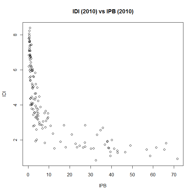
IDI decreases at a decreasing rate with respect to IPB.
A regression model was fitted to quantify
this relationship.
Regression
model output:
Call:
lm(formula
= log(IDI2010) ~ log(ICTpricebasket2010))
Residuals:
Min
1Q Median
3Q
Max
-0.71750
-0.12492 0.02376 0.15908
0.49380
Coefficients:
Estimate Std. Error t
value Pr(>|t|)
(Intercept)
1.80628
0.02599
69.50
<2e-16 ***
log(ICTpricebasket2010)
-0.36628 0.01267 -28.92
<2e-16 ***
---
Signif.
codes: 0
‘***’ 0.001 ‘**’ 0.01
‘*’ 0.05
‘.’ 0.1 ‘ ’ 1
Residual
standard error: 0.2221 on 143 degrees of freedom
(7 observations deleted
due to missingness)
Multiple
R-squared: 0.854,
Adjusted
R-squared: 0.8529
F-statistic:
836.2 on 1 and 143 DF, p-value:
<
2.2e-16
For those who aren’t familiar with regression
output:
The high (close to one) R-squared statistic shows that the
model fits strongly to the data:
Multiple
R-squared: 0.854
The very low (close to zero) p-values, show that the parameters of the
model are highly significant:
Pr(>|t|)
<2e-16 ***
<2e-16 ***
These figures are the coefficient estimates, used to
construct the model.
Estimate
(Intercept) 1.80628
log(GDPpcppp2010) -0.36628
The fitted model is
represented by the following equation:
Where:
x is the
IPB
y is the
IDI
The
fitted regression model curve added to the
plot:

The two variables are interdependent.
The lower the price of information and communication
technologies (relative to income), the more affordable it is to
adopt those technologies, resulting
in a higher quantity of demand for them (resulting in a higher IDI).
The development of information and
communication technology infrastructure results in an increase in
supply,
resulting in lower prices for information and communication
technologies.
IDI Combined Model
A regression model was constructed which includes both IPB
and GDP per capita (PPP).
The model has the following structure:
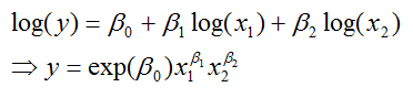
where:
y is the IDI
x1 is GDP
per
capita (PPP)
x2 is the IPB
Regression
model output:
Call:
lm(formula
= log(IDI2010) ~ log(GDPpcppp2010) + log(ICTpricebasket2010))
Residuals:
Min
1Q Median
3Q
Max
-0.63013
-0.11554 0.01074 0.12034
0.54496
Coefficients:
Estimate Std. Error t
value Pr(>|t|)
(Intercept)
-0.97586
0.38346
-2.545
0.0120 *
log(GDPpcppp2010)
0.27327
0.03755
7.277 2.23e-11 ***
log(ICTpricebasket2010)
-0.15858 0.03139 -5.052 1.34e-06 ***
---
Signif.
codes: 0
‘***’ 0.001 ‘**’ 0.01
‘*’ 0.05
‘.’ 0.1 ‘ ’ 1
Residual
standard error: 0.1862 on 140 degrees of freedom
(9 observations deleted
due to missingness)
Multiple
R-squared: 0.8984,
Adjusted
R-squared: 0.8969
F-statistic:
618.7 on 2 and 140 DF, p-value:
<
2.2e-16
The fitted model is
represented by the following equation:
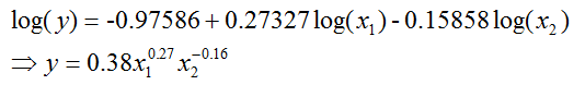
where:
y is the IDI
x1 is GDP
per
capita (PPP)
x2 is the IPB
The combined model is similar to the constant price elasticity
demand model used in econometrics.
A
constant price elasticity demand model would have the logged quantity
(or
logged expenditure) explained by the logged price and other variables
that
explain demand, including a variable related to income.
The coefficient of the logged price explanatory
variable is interpreted as the price elasticity of demand i.e. a 1%
increase in
price, would result in a percentage change in the quantity demanded on
average equal
to the coefficient estimate.
Download the Data Set
The data set containing the IDI, IPB and GDP
per capita (PPP) data
can be downloaded here.
Note that:
- If a country doesn’t have an IDI figure but
did have an IPB
figure, they weren’t included in the data set.
- Some countries don’t have IPB values.
- There were more missing IPB values for 2008 than for
2010.
- There are missing values in the GDP
per capita (PPP) data.
- Some of the GDP
per
capita (PPP) figures are
from before 2010.
External link:
ITU Measuring the Information Society
See
also:
Regression
|


